Negotiation Leverage and the Massive Hidden Value in ELC/RFA Deals

This article is being co-posted on Maple Leafs Hot Stove as well as on my own site, http://www.originalsixanalytics.com. Find me @michael_zsolt on twitter.

Recently I completed a three-part series on the Wins Above Replacement (WAR) and Goals Above Replacement (GAR) metrics. In it, I summarized how the GAR metric can be used for player evaluation, how it can be used to calculate player value, and how GAR can be used to derive an entire team’s salary cap ‘efficiency’. I’d like to add one last bonus article to the series to touch something I have often mentioned: the huge importance of Entry Level Contracts (ELCs) and Restricted Free Agency (RFA) years in a salary capped league.

In this piece, I will touch on (i) the impact of negotiation leverage on contract discussions, (ii) how to quantify the value of ELC and RFA deals to teams, and (iii) a short review of these things in practice, by looking at Steve Yzerman’s impeccable handling of Jonathan Drouin’s trade request situation. By the end, I will hopefully demonstrate the immense amount of value for teams that ELC/RFA contracts can create – which further establishes the importance of building through the draft, as well as generally acquiring players at the very early stages of their careers.


Market Dynamics and Negotiation Leverage

How negotiation leverage impacts transactions (e.g. trades, contract signings) is something I think most people understand intuitively. Whether inside or outside professional sports, in any transaction the buyer wants to minimize the price paid for an asset, and the seller wants to maximize it. The way market dynamics play into this is driven by the options available to both parties. If a seller has a scarce asset, and can get 5-10+ interested potential buyers (e.g. resembling an auction), the seller is in a position of strength, and will likely get an excellent return. This can even hold true with as few as two or three serious buyers. However, if a buyer is somehow able to get into an exclusive, one-on-one negotiation with a seller, that buyer instead holds significant leverage, especially if the seller is ‘forced’ to get rid of the asset.

Although this is true in every-day scenarios (e.g. to get a good price, it is better to look at three retail stores when buying a new TV, not just one), a great example of the market dynamics side is buying a house. Toronto’s housing market is currently quite ‘hot’ – with 5+ buyers bidding on most houses – as a result, almost every single one trades for a premium to its asking price. Like I said –intuitively, I think we all already know these fundamental concepts.

Now, in the case of hockey, there are two primary situations where negotiation leverage becomes important:

  1. Player-Team negotiations
  2. Team-Team negotiations

For what it’s worth, NHLPA-NHL negotiations also take place, essentially being Player-Team talks at the level of the entire league.

In this article I will be focusing on team-player negotiations, in particular on the substantial impact that ELC/RFA constructs have on them. However, for those interested, my last post touched on the team-to-team side briefly, discussing how the strong trade deadline demand for defensemen and weak demand for goalies impacted the Leafs’ yield on Roman Polak and James Reimer, respectively.

How do Entry Level Contracts (ELCs) and Restricted Free Agents (RFA) Work?

Before quantifying the value of the ELC/RFA concepts, I will give a brief summary of how they work, simplifying it into three categories: (a) ‘ELC’ deals, (b) ‘RFA’ deals, or (c) ‘UFA’ deals (Unrestricted Free Agent) – driven by age at signing and years played in the league. However, keep in mind this is a high level summary, as these concepts fill a number of sections in the Collective Bargaining Agreement (CBA), and free agents are actually divided into six distinct categories. For those who want a very detailed walk through of these concepts and the rest CBA, I recommend you check out @JJfromKansas’ great 2013 series Getting to know the CBA’.


At a high level, Entry Level Contracts:

  • Apply to players in their first three seasons in the league, with seasons defined different depending on the player’s age
  • Also typically expire when a player turns 25, if that player has not yet reached three seasons
  • Limit players’ base salary to a maximum of $975K, or a cap hit of $3.8M after including possible performance bonuses (regardless of if those bonuses are paid)
  • Cannot include no-trade/no-movement clauses, and must be two-way contracts

Following a players’ ELC, they enter Restricted Free Agency. RFA players:

  • Will be an RFA either until they turn 27, or until they have played 7 professional seasons
  • Are only able to negotiate with the team that holds their exclusive rights
    • Other teams can extend RFAs an ‘offer sheet’, but generally (i) the current team can match it, or (ii) the current team will be compensated by the ‘poaching’ team with draft picks
    • Compensation ranges from a third round pick for players earning $1.1M-$1.6M per year to four first round picks for players making $8.4M+ per year
  • Also prohibit no-trade/no-move clauses during RFA years
  • Last, as long as teams extend RFAs a ‘qualifying’ offer, players have limited leverage in the negotiation, with the exception of invoking (or threatening to invoke) arbitration

Unrestricted Free Agents (UFAs) are just that – the first time a player can ‘test’ his value on the open market, unencumbered by the CBA. For what it is worth, I currently have no strong view on if this system is fair or not – as of right now, these are the rules of the game, so they are what they are.

ELCs/RFA deals are specifically designed to give teams negotiation leverage over players early in their careers – with ELCs putting a direct cap on that player’s salary, and RFA’s implicitly stifling their compensation by forcing them into one-on-one negotiations.

To be clear, just based on the ever-increasing value of draft picks in trades, all GMs already know that these ELC/RFA years are hugely valuable – this is not an innovative or original concept. However, what is less clear is whether many NHL teams understand exactly how much these rights can ultimately be worth to them.

As such, I now want to attempt to answer:

What Are a Players’ Exclusive Negotiating Rights Worth to a Team?

We won’t be able to get an ‘exact’ answer to this question, because it is a very theoretical concept and is entirely dependent on which actual players is being discussed. As a result, I will instead use an illustrative example that shows – for a particular set of players – how much value they contributed to their respective teams over each of their ELC/RFA/initial UFA years in comparison to how much they were paid in that time. The method I will use to determine what a player is ‘worth’ is the exact same as I used in my previous articles, so I encourage you to check those out if the math is unclear.

To start, I selected a sample of elite-level players, to illustrate the extreme end of the spectrum in terms of contribution to their teams. I selected 10 forwards from across the league who have (almost all) reached the UFA portion of their contracts. Here is the sample I looked at:

Table

First, I stacked up all of these players next to each other in terms of their annual salary cap hits (Average Annual Values, or AAV), with data from General Fanager.  Here is the group’s average AAV per player over their first 10 NHL seasons:1 - AAV

(Note: Although players become UFAs after seven years played, all of the players listed were signed to at least a five-year deal when their ELC expired. As a result, teams earned the savings on these players’ contracts up until their 8th NHL seasons, and I have treated their 8th season as a year locked into an ‘RFA’ contract)

Just from this you can already see the huge impact that ELC and RFA years have on a players’ compensation – these guys are the equivalent of slave labour in their first three seasons, when compared to their contributions/value.

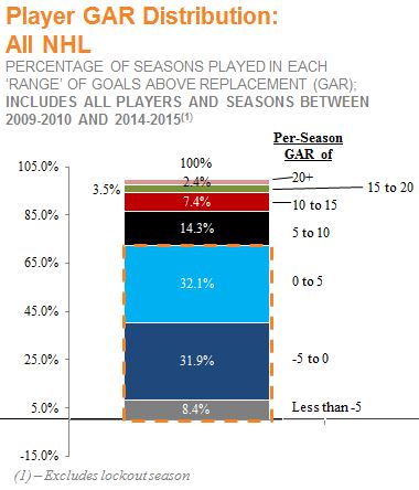
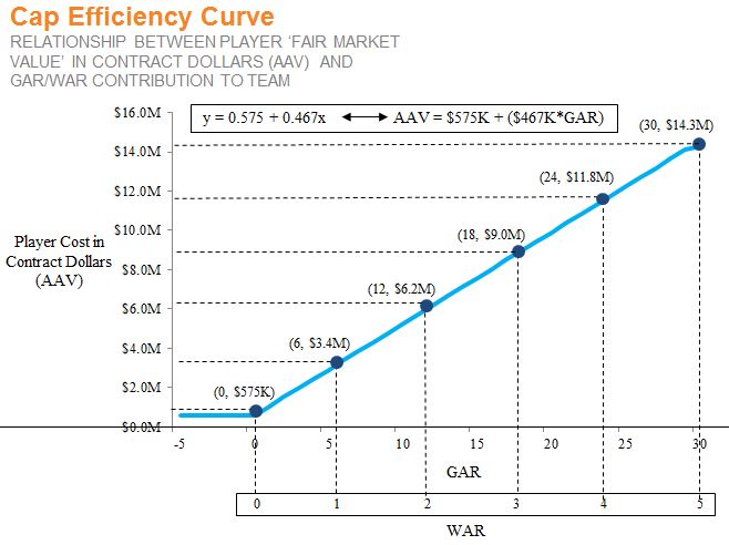
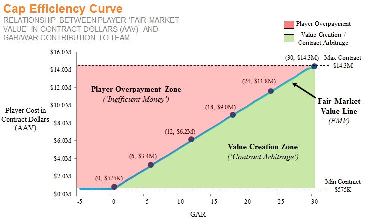
Next, in order to derive what these players are worth to their respective teams, I calculated their average annual GAR contributions, as well as what those GAR values should be worth based on Hawerchuck and Eric T’s relationship between WAR/GAR and contract dollars (e.g. AAV FMV =$575K + ($467K * GAR)).2- GAR3 - FMV(Note: For the players who had not yet reached 8-10 seasons of data, I estimated the last couple years of GAR data based on that player’s 3-yr Avg GAR, and the player’s UFA AAV was treated as equal to their FMV – this was only the case for one or two players)

Last – I calculated the amount teams’ saved, on average, in each year of these players’ contracts. In short – this was done by subtracting the average actual AAV (e.g. Chart #1) from the value contributed / FMV of these players to their teams (e.g. Chart #3, above). Here is the result, on both an individual year and a cumulative basis:

4 - Value Created5 - Cumulative Value

Now – I think this tells us a very interesting result: for the contribution made by this type of elite, franchise player, the combination of ELC and RFA years equate to almost $27M in salary cap dollars saved by their teams. Further, the vast majority of this is driven by ELC years – players get only slightly less than FMV in their 4 or 5 RFA seasons. I don’t know about you, but I was a bit blown away by the huge amount of value this can create for teams.

And again – to be clear – because these are 10 of the highest-performing players in the league, this illustrative analysis shows essentially the maximum that ELC/RFA years could be worth, not the league average, nor what ELCs/RFAs will even ‘usually’ be worth. The other end of the spectrum – replacement level players who make the league minimum salary ($575K per year) – there is little to no incremental value in these years, as those players are not commanding premium prices in the first place.

Negotiation Leverage in Practice: Jonathan Drouin vs Tampa Bay Lightning

Finally, I want to bring this all together in a specific example, where Steve Yzerman (GM of Tampa Bay Lightning) demonstrated a clear understanding of his own negotiating position, as well as of the value of ELC/RFA deals in his recent interactions with Jonathan Drouin. For those who don’t know, Drouin is a former 3rd overall pick, still on his entry level deal, who was apparently having issues with Jon Cooper, Tampa’s head coach. As a result, Drouin privately requested a trade at the beginning of the season, and went public with his request in early 2016. In January, Drouin was then sent to Tampa’s AHL affiliate, the Syracuse Crunch, where he eventually chose not report to play, and was subsequently suspended by his team. As the trade deadline approached, Drouin was the subject of many trade discussions – with other teams in the league likely trying to take advantage of Yzerman’s seemingly ‘forced seller’ position, presumably giving him slightly ‘low-ball’ offers  for the young star.

However, it is now clear that Yzerman fully understood his negotiating position and level of control over the situation as it was unfolding. Further, he seems to have had the foresight to avoid setting a precedent that if a player (with zero leverage) were to complain enough, that the team would ultimately cave. Based on the analysis above, I would guess that Yzerman knew very well that he had up to $27M in salary cap efficiency he was going to lose if he dealt Drouin for less than his fair value – so his ask from other teams was rightfully high. As a result, no team stepped up with a good enough offer, and Tampa Bay kept Drouin at the deadline – fully understanding the risks.

Now, with the recent news this past week, it appears the situation has come full circle. Drouin has apparently realized that Yzerman is no push-over, and if he ever wants to play hockey in the NHL again he will have to do so as the Tampa Bay Lightning see fit. Lo and behold, earlier this week Drouin approached Yzerman about being willing to play for the Syracuse Crunch, has reported to the team, and apparently even had conversations about Drouin possibly coming back into the fold for Tampa’s playoff run. Although we knew Yzerman’s trade ask was high, many observers likely thought that the pressure on Yzerman was so great that he would be ‘forced’ to off-load Drouin at below his fair value. Instead, Stevie Y recognized his leverage in the situation, stood his ground, and either will reclaim one of his top prospects, or at least be able to trade him for full value in the future.

Well played, Steve.

PS – Here was my take on the situation back in January, shortly after it was announced that Drouin had refused to play for Tampa’s AHL team, in an effort to force Yzerman’s hand to trade him:

Tweet1

Tweet2

Tweet3

Tweet4

Tweet5

Tweet6

Conclusion

Hopefully this provided an interesting look at how negotiation leverage impacts contract situations, the huge value of ELC and RFA deals to teams, and also a useful example of this playing out in reality. In the end, it should now be clear that there is a huge amount of hidden value in getting a player at the front end of his ELC/RFA years – up to $27M, in fact. Last, I think it is clear that Steve Yzerman has successfully sent a message to his players, and potentially the league, that they are a team with a clear understanding of these two concepts, they are steadfast negotiators, and especially when they find themselves in a position of strength – Tampa Bay is not an organization to that will be pushed around.


The Model Franchise: GAR, Roster Construction, and Maximizing Team-Level Cap Efficiency (Part 3)

 (OSA’s WAR “Explainer” Part 3)

This article is being co-posted on Maple Leafs Hot Stove as well as on my own site, http://www.originalsixanalytics.com. Find me @michael_zsolt on twitter.

Thus far in my Wins Above Replacement (WAR) ‘Explainer’ series I have covered:

  • Goals Above Replacement (GAR) & Player Evaluation, and
  • Using GAR to Quantify Player Value & Salary Cap Efficiency

Now, for the final post in the series, I’d like to show how GAR can be applied to team level decisions. First, I will show some analysis done by Moneypuck to demonstrate the relationship between GAR and standings points. Second, I will look at the 2014-2015 Chicago Blackhawks and Toronto Maple Leafs to show (i) a textbook example of using GAR to guide a team’s roster construction and salary cap management and (ii) what happens when a team ignores it altogether. Last, using the 2000-2015 Chicago Blackhawks as the best example of a modern ‘Model Franchise’, I will show how Brendan Shanahan’s Leafs’ organization seems to be borrowing a few pages from the Blackhawks’ playbook of the last decade.

Why GAR is Important for Roster Construction

Last summer, Moneypuck did some excellent analysis where he demonstrated the very strong relationship between a team’s total GAR score and its points in the standings – even stronger than Corsi. I borrowed the chart below from Moneypuck’s analysis, showing how a team’s GAR score for a season on the x-axis can be a driver of its total points, on the y-axis.

Moneypuck image

Source: http://canucksarmy.com/2015/8/17/how-to-build-a-contender-part-1-war-what-is-it-good-for

Here is a summary of his findings:

  • Based on the R2 above, GAR has the ability to predict roughly 72% of how a team will end up in the standings (retroactively)
    • This compares to ~38% predicted by 5v5 Corsi%
  • Using this equation, a team with a total GAR of zero – the same as a hypothetical ‘replacement level’ team – would score roughly 76 points in the standings
  • Adding players above/below replacement level to a team would conceptually ‘move’ that team’s expectations up or down the curve shown, based on that players’ GAR

Moneypuck then split up all conference finalist teams since 2009 by GAR score, and had some pretty clear findings:

Moneypuck chart

Note: All GAR data original ly comes from WAR-on-ice.com, and the contract information from charts later on comes from Rob Vollman’s 2014-2015 comprehensive stats database.

The chart above shows that, although Cinderella stories do take place, 80% of conference finalist teams have total GAR scores of 107 or more. This analysis can almost be said to define the ‘goal posts’ of how GAR can be used for roster construction.

Based on this, NHL GM’s could reasonably set a target of 107 GAR for their teams. In years where a team is forecasting close to 107 GAR, the GM should consider trading for those last 1-2 key pieces to make a run. If the team is well off of 107, the GM can instead use it to guide his long term plan by answering (i) how he can acquire a core group of players to reach 107 GAR, and (ii) once acquired, how can he best divide his cap space between those players in order to keep them?

Now that the goal posts are established, I will look at team-level cap efficiency and roster construction of our two example teams: the 2014-2015 Blackhawks and Leafs, based on their season-end rosters.

Team-Level Salary Cap Efficiency

First, I will revisit the Cap Efficiency Curve from my last post, but for a whole team at once, rather than for just a single player. I encourage those who haven’t read my last two articles to go check them out, as it will provide the necessary context for the upcoming analysis.

Hawks - Arbitrage line

Looking at the above, you can observe the following:

  • Almost all Chicago players are on or to the right of the ‘zero GAR’ line – that is, almost all have contributed more than replacement level
  • Relative to the Fair Market Value (FMV) line, Chicago has players both on value-creating and over-paying contracts
    • However, most players don’t stray too far from their FMVs; generally the team slants upward and to the right, with the highest pay going to the greatest contributors
  • The most notable exceptions to this pattern are:
    • Brent Seabrook, who has weaker shot-rate contributions than you would expect, a major driver of GAR
    • Jonathan Toews, who was in his last RFA year in 2014-2015 (which also explains the 2016 bump to 10.5M, shown in my last article)
    • Brandon Saad, who was finishing his ELC in 2014-2015, was understandably traded to Columbus once he came due for a raise in the offseason; the Blue Jackets promptly signed him for 6 years at $6M per year

Now – let’s compare this to the 2014-2015 Leafs:

TML - Arbitrage line

Here, you can make largely the opposite observations:

  • Many Leafs players are on the wrong side of the zero GAR line, putting them below replacement level over this period
  • There are very few examples of players in the ‘green’ area of the chart, with only Kadri, Bernier and Panik having value-creating contracts
  • For what it is worth, this under-sells some players: e.g. Morgan Reilly is being dragged down here by his rookie and sophomore seasons, a time when few players will score well on GAR

Value Creation / Overpayment by Individual Player

We can also look at this output as the actual dollar value created (or overpaid) for each individual player; similar to what I did for Toews, Phaneuf, Parenteau and Boyes previously. I calculate this by subtracting each player’s contracted AAV from the AAV of the FMV line, at the same GAR score. Green bars represent value being created for the team, while red bars represent value lost/overpaid to the player.

Hawks - by player calc

The Hawks’ results here are consistent with the earlier chart, where Saad, Toews and Seabrook were the most extreme examples in an otherwise balanced group. This chart also shows:

  • The Hawk’s 3-year Avg Team GAR was 105.6 – just what you would expect of a conference finalist/Stanley-Cup winning team
  • The team’s net total value overpaid was -$6.3M
    • This represents the approximate year-end cap hit of the Blackhawks at ~$69.9M(1), minus the total FMV of their players at $63.6M

(1)- Slightly off of year-end total due to timing

Although the Blackhawks slightly ‘overpaid’ their players according to this analysis, more broadly I think the Hawks were generally quite close to paying players the appropriate amount across the board.

However, what this result tells me is that a big part of effectively managing a roster will come down to simply not overpaying players. It is extremely hard to find a player that can be signed for less than he is worth, largely happening only when the player is drafted and held for all of his ELC/RFA years. As a result, the simplest way a team can effectively manage its salary cap is to be disciplined in contract negotiations, and avoid giving large contracts to high risk or potentially declining players.

Speaking of overpaying players…

TML - by player calc

This chart shouldn’t need much explaining. Nazem Kadri is the sole shining light of the Leafs’ from last season, and Phaneuf was the largest contract drag they (previously) had on the books. (Note – This was supposed to be based on season end roster but somehow guys like Holzer snuck in there).

Applying GAR Directly to Roster Construction

Last, I will look at how teams like the Blackhawks allocate cap space when constructing their rosters. Specifically, I will compare the percentage of the cap that each player receives in pay, as well as the percentage of the team’s GAR that each player contributes. Any team that is applying this type of thinking to its roster construction would ideally attempt to match these two percentages closely, so as not to ‘waste’ cap space on non-contributing players.

Not surprisingly, that is exactly what we see from the Blackhawks:

Hawks - roster construction

  • The chart above shows a very interesting, and potentially deliberate matching of a player’s GAR contribution and his portion of the cap earned
  • Many of the Blackhawks’ largest GAR contributors have slight greater GAR percentages than cap percentages, again suggesting the Hawks are getting good returns on their dollars
  • Last, this chart helps to show that the Blackhawks have constructed their roster around a ‘core’ set of 7-8 players that drive their results:
    • This core consists largely of the team’s top 4 forwards, top 3 defensemen, and starting goalie (Toews, Kane, Hossa, Sharp, Keith, Seabrook, Hjalmarsson, and Crawford)
    • These players collectively earn 64% of the salary cap, and contribute 67% of the team’s GAR
    • Interestingly, this directly matches the typical conference finalist team having ~8 or so 10+ GAR players, shown in Moneypuck’s analysis cited in my first article

This chart is relatively clean and easy to read, in part due to how well the Hawk’s connect their cap hits to player’s GAR. The Leafs, unfortunately, had a lineup that was mixed between players with positive and negative GAR scores – making this type of analysis less clear and intuitive. To make up for this, I have split the Leafs’ team GAR chart into two sub-charts, one for each of the team’s positive GAR players and its negative GAR players, with each group separately totaling to 100%. Note: as a result, the percentages of the positive and negative bars are not directly comparable to each other.

TML - roster construction

A few comments:

  • Almost 60% of the Leafs cap space was going to players who were contributing zero or negative GAR value to the team
    • 15% of this was also driven by their surprisingly high, non-contributing $10.5M of bought out and retained cap space
  • As mentioned, the Leafs’ net GAR score is 19.5, or the difference between positive GAR players of 43.9 and the negative players of -24.4
  • The Leafs ‘core’ players were simply not of the same caliber or ability to drive a team’s results as the core on the Hawks

In the end, it is clear this type of analysis was not driving the roster construction decisions of the legacy TML front offices. Instead, the lack of it helped to dig the giant salary cap hole that Shanahan inherited.

Building ‘The Model Franchise’ In Toronto

Although the Leafs entered 2015-2016 in a difficult position, the last 8 to 10 months have given fans ongoing reasons to be optimistic about the future. As such, I will close out by touching on five major parallels between the 2000-2015 Chicago Blackhawks organization, and what Brendan Shanahan has begun to do to fulfill his vision of “returning an original six franchise to its rightful place in the league”.

  1. Front Office & Coaching

Under GM Stan Bowman, head coach Joel Quenneville, and with a senior advisor of the winningest coach in NHL history, Scotty Bowman, the Chicago Blackhawks easily have one of the best front offices in the league. Over the last two years, Shanahan has done an unbelievable job putting together a team of arguably the same caliber: between Lou Lamoriello, Mike Babcock, Mark Hunter, and Kyle Dubas, the Leafs’ have an equally all-star leadership team. It is also worth noting the similarity between Babock’s and Quenneville’s system-driven styles, which are both centered on driving puck possession.

  1. Building Through the Draft: Quantity First

Between 2000 and 2004, the Chicago Blackhawks had the highest number of picks of any team in the league at 64, versus the league average in that period of 48, and the next highest of 58. This allowed them to pick up many core pieces they still have, long before Toews & Kane arrived (e.g. Keith (2nd round), Crawford (2nd round), or more recently, Saad (2nd round). As I discussed in a previous article, the Leafs are employing a similar strategy, both by maximizing the quantity of their picks, and also by hopefully leveraging Mark Hunter’s strong scouting organization and network.

Separately, to the concept of ‘building a core 7-8 players’, many fans have enjoyed speculating that the Leafs’ major recent draft picks of Nylander, Marner, Reilly, Kadri, (as well as Gardiner, who they traded for) etc., will make up that group going forward. Only time will tell.

  1. Investing in Player Development

Both teams focus on managing their organizations holistically, by working closely with all of NHL, AHL, and often ECHL rosters. Like Babock’s former Red wings, both teams also push players to develop in the minors, with even two-time Norris Trophy winner Duncan Keith having spent two years in the AHL. The Leafs also lean on the Marlies to help young players learn the team’s system, and help the entire organization focus on every player’s development at both levels. Finally, building a large pipeline of young talent through the draft also allows both the Hawks and Leafs to hold those players on very beneficial contract terms for approximately seven seasons while players play through their ELC/RFA years.

  1. Global Scouting & Free Agents

Finding elite talent is a very difficult task, and the most successful organizations leave no stone unturned. The way Chicago’s was able to pick up a first-line player like Artemi Panarin as a free agent signing (also currently on an ELC deal) is the NHL-equivalent of found money. Although Nikita Zaitsev will not necessarily be of the caliber of Panarin, if the media is right that Zaitsev plans to sign with the Leafs at seasons’ end, he will no doubt be a major player to land. The potential to pick up a developed, 24 year old potential top four defensemen provides even more strong evidence in support of investing in scouting around the globe.

  1. Strategic Cap Management & Roster Construction

Last – although the analysis above shows Shanahan and company have inherited a very unfortunate roster situation, they are clearly doing the right things to slowly off-load anchor contracts, sign value-creating free agents, and offload pending UFA contracts for future assets in picks and prospects. I think it is safe to say that two or three years from now, the Leafs’ roster and salary cap situation will look a lot more like that of the 2014-2015 Chicago Blackhawks’ than it resembles the Toronto Maple Leafs team that Shanahan inherited.

Conclusion

With that, I will wrap up my ‘WAR Explainer’ Series – so thank you to those who have made it through all three parts. In it, I have covered (i) GAR & Player Evaluation, (ii) Player Value and Contract Efficiency, and (iii) GAR and Roster construction/Team-Level Cap Efficiency. Hopefully the series has also provided an interesting view into how the current Leafs’ organization is implementing these principles in their long term rebuild, and helped us all build our patience a little longer. Maybe, just maybe, 5-10 years from now fans will be looking back at the Shanahan-Era Toronto Maple Leafs as the modern NHL’s next Model Franchise, to be emulated for years to come.

Using GAR to Quantify a Player’s Value and Salary-Cap Efficiency (Part 2)

(OSA’s WAR “Explainer” Part 2) 

This article is being co-posted on Maple Leafs Hot Stove as well as on my own site, http://www.originalsixanalytics.com. Find me @michael_zsolt on twitter.

In my last article I walked through what the WAR/GAR metric is, and the practical applications, and limitations, of using it to evaluate individual players. In this post I would like to build on that work to (i) show how to use GAR to quantify what a player is worth in dollars, (ii) introduce the concept of ‘contract arbitrage’, and (iii) use that concept to review the cap efficiency of Jonathan Toews, Dion Phaneuf, P.A. Parenteau and Brad Boyes.

GAR and Quantifying Player ‘Value’

In a salary-capped league, NHL franchises operate under a series of constraints:

  • Maximum of 50 contracts per team
  • $71.4M salary cap in 2015-2016
  • $52.8M salary minimum
  • Minimum NHL-level salary of $575K
  • Maximum NHL-level salary of $14.3M (20% of the cap)
  • Maximum Entry Level Contract (ELC) base salary of $925K, or $3.78M after performance bonuses

As you can see, the Collective Bargaining Agreement (CBA) defines the limits that teams must optimize within. When faced with this, the concept of opportunity cost becomes extremely important. Opportunity cost is the implied cost of a decision by not choosing the next-best alternative available at the time. Think of signing a 35+ year-old to a five-year, $35M deal. Even if that player is a strong contributor, the team’s opportunity cost (five years of losing ~10% of their cap) will often make these deals unjustifiable, especially as that player’s performance declines over time.

Having looked at GAR and player evaluation, I now want to incorporate contract dollars to show how to use GAR to quantify player ‘value’. To do this, I will be focusing on salary cap impact (rather than annual salary paid), as that is what matters to teams when making contract decisions – at least those that aren’t more constrained by their own finances than the cap (e.g. ‘budget’ teams). As you may know, salary cap hit is calculated by the league as the average annual value (AAV) of a player’s contract.

The central approach I will be using to value players is based on some very helpful past analysis by Eric T and Hawerchuk. Amongst many other things, their work showed us the following:

  • 1 win (WAR) = ~6 goals (GAR)
  • Based on the free agent market and the current cap, every 1 WAR a player contributes is worth $2.8M in contract value
  • After adding in the baseline salary ($575K minimum contract, AKA a zero-GAR player): the market ‘price’ of a 1 WAR or 6 GAR player is approximately $3.4M in player salary per year

Estimating Player Value: Some Initial Examples

One way to connect our $2.8M cap-dollars per win to players is to simply insert it into the table I shared in my last post. Doing so will give a range of estimated player ‘value’, shown in terms of contract dollars against the cap.

Expected Contract Dollar by WAR Range

Hopefully this table helps demonstrate an initial idea of what these players are ‘worth’, based on their GAR scores. However, much like my previous draft-pick-value analysis, what works well for a range is not necessarily as applicable on an individual basis. Instead, showing this on a curve can help us assign players a more precise estimate of the value they contribute, and deserve.

The Cap Efficiency Curve

To demonstrate this, I have created the chart below, which I will call the ‘Cap Efficiency Curve’. This curve illustrates the linear relationship between a player’s cost (in contract AAV) and the GAR/WAR a team should expect from an individual with that level of compensation:

Player Value vs Cost Curve

The relationship shown above is relatively straightforward, directly derived from our earlier concepts – that each 1 WAR/6 GAR is worth $2.8M in AAV, above the player’s minimum salary. Hopefully this visualization can help turn the general relationship into an intuitive, usable tool for a team. For example, this curve allows us to:

  1. Evaluate if a player is outperforming/underperforming expectations in his existing contract
  2. Define the ‘fair’ market price for a player’s future contract, based on what he has been able to do historically, and ideally, based on what we can project he will do in the future

One note: as you can see, the equation above only holds between the minimum and maximum player salary levels, as a player currently cannot be paid less than $575K or more than $14.3M per season.

Now that we have a good understanding of what a player is worth – how can a team leverage this relationship to ensure they use their cap space as efficiently as possible?


‘Contract Arbitrage’: How to Take Advantage of Market Inefficiencies

The word ‘arbitrage’ can have multiple meanings, depending on whether it is being used in a very technical, financial sense, or a more general one. More generally, people use arbitrage to mean buying something for less than it is worth. Like a typical ‘value’ investor, this is done by conducting detailed research to figure out an asset’s ‘true’ value, before searching for opportunities to acquire it at a very good price. After purchase, value investors typically hold assets (companies) for a very long time, often continuing to invest their dollars, time and expertise in order to maximize future growth, profits, and investment returns.

Applying this value investing arbitrage to the world of NHL contracts brings me to the idea of ‘Contract Arbitrage’. I will define ‘Contract Arbitrage’ as any situation where a team receives more value from a player’s contract than it costs them. Specifically, that would mean earning more in WAR/GAR than the team gave up in equivalent cap-space, making contract arbitrage a measure of cap-efficiency as much as it is ‘financial’ value. While GMs are most obviously focused on acquiring talented hockey players, a key component of the job of a GM is to maximize his team’s wins per cap dollar spent.

Let’s go back to the Cap Efficiency Curve to illustrate this concept:

Value vs Cost Curve - ShadedLooking at the above:

  • Fair market value (FMV) for a player would be any contract value along the curve shown
  • Overpaying for a player would be a contract that falls into the area above the curve (shaded red)
  • Creating value (e.g. signing a player with the potential for contract arbitrage) would be any contract that falls into the green area, below the curve
    • Simply put, the green area represents any time a team pays a player less than the goals/wins he contributed to the team would justify

For simplicity, I will focus my upcoming examples on past performance, in order to illustrate these concepts. In the truest sense, teams should be using this concept on a forward-looking basis. For example, if a team can reasonably forecast a 20-22 year old to reach 10, 15, or 20+ GAR over the next 5+ years, they should be inclined to ‘lock in’ his contract now – ideally within the green area of the chart above. Keep an eye on Aleksander Barkov’s GAR performance over the next few years, as he may grow into an excellent example of such a contract.

Now – let’s get into those examples:

Our Original GAR Case Study: Jonathan Toews

I will start with Jonathan Toews in order to connect this analysis back to the player evaluation case study from my last post. Toews’ 3-year average GAR is 20.3, and his current AAV is $10.5M on a contract with seven years remaining. Plotting Toews’ GAR together with his contract dollars on the curve below will help us see if he is currently being over, or underpaid. The curve will also allow us to see how much over/underpaid Toews is – measured by the distance between his (x,y) coordinates and the FMV line.

Contract Eval - Toews

  • As shown above, plotting Toews’ onto the Cap Efficiency Curve shows he is ‘worth’ ~$10.1M (e.g. where his ~20 GAR hits the curve)
  • Compared to the $10.5M AAV he currently takes of the Blackhawks’ cap, this would show Toews’ to be paid quite close to his fair value, receiving a ‘premium’ of only $400K

Although Toews’ performance has started to show slight declines, I would argue that Toews’ contract appropriately reflects his FMV. Teams will never be able to predict exactly how a player will perform, but the Blackhawks have come pretty close here. Further, this calculation doesn’t attribute any value to qualitative factors, such as the incredible leadership, work ethic, and experience that Toews brings to his team. In my view, these factors will more than offset the $400k premium that the Blackhawks are paying.

Now let’s look at an example at the opposite end of the spectrum…

Former Toronto Maple Leaf: Dion Phaneuf

First, I want to go on the record and say that I had written almost this entire article and analysis of Dion prior to the recent announcement of his trade to the Senators. As a result of that announcement, I now get the benefit of no longer explaining to the world just how bad Dion’s contract is for the Leafs, and how hard it will be for them to offload it. So that is nice.

Second, I will deliberately avoid getting too far into reviewing the trade directly, as there are many other good examples of people who have done so already. My big picture ‘take away’ is that I was very impressed by the Leafs’ ability to source and negotiate a deal that rids them of his contract, with zero salary retained. I also will say that, from the seat of a Leafs’ fan – i.e. supporting a team that has always been overflowing with cash, and is only constrained by the cap – it can be hard to appreciate this deal from the Senators’ perspective.

However, I think the swap has more positives for the Senators than most think. In this trade, the Sens found a creative way to convert very unproductive cap space (injured/inactive players) into a contributing asset (Dion) with a similar cap hit, only for a longer term. Further, James Mirtle’s insightful tweet summarized that the Sens’ actual cash out the door for next season went down by $4.2M after this deal. For a budget team, that cash compensation change is arguably just as valuable as offloading an additional $4.2M in salary cap – all while picking up a solid, top 4 defensemen.

Now – let’s take a look at Dion’s contract.

Contract Eval - Phaneuf

  • Plotting Dion’s $7M AAV and his 3-year average GAR of -3.4 (2012-2013 to 2014-2015) paints a dismal picture
  • Relative to the FMV line, Dion is being paid $6.5M per year more than he contributes to his team’s goal differential
  • The most pessimistic way of looking at this (which I’m sure will make most Leafs’ fans glow), is to directly multiply the $6.5M loss by the five remaining seasons on his deal: giving a total maximum overpayment/loss of value of $32.5M

However, much like we couldn’t reasonably interpret the first graph as simply ‘Toews is overpaid’, I think we need to caveat this analysis for Dion as well – even if that only results in being nice to Sens fans. To qualify this analysis of Phaneuf’s contract:

  1. First, as shown in my last post, GAR doesn’t necessarily include every aspect of how defensemen contribute to their teams – thus, it may understate the value of Dion, or any other D-man
  2. Second, this data also only includes up to 2014-2015; the eye-test alone makes it clear that Phaneuf has stepped up in the current 2015-2016 season. The change in Dion’s usage and minutes under the Babcock regime have likely bumped up his recent GAR considerably – and to Ottawa’s credit, they were buying into Dion’s play this year, not his play over the three years before this one
  3. Last – I legitimately believe Lamoriello and Babcock’s comments that Dion is an excellent leader, person, and guy to have in the Leafs’ dressing room. I think this was providing a lot more value to the Leafs than us number-crunchers tend to give credit for – and it will be missed

Going forward, the same analysis above can be applied to see if Dion is living up to his contract any better in the future than he has historically. By tracing his $7M over to the FMV line, we can see that a $7M AAV player ought to be in the 13-14 GAR range each year. Thus, if Dion’s GAR for 2015-2016 and onward come out anywhere north of 10, Ottawa will be looking a lot better than we all are currently giving them credit for.

For one last example, let’s look at the free agent signings done this past summer by the Leafs’ current front office:

Brad Boyes and P.A Parenteau

Brad Boyes and P.A. Parenteau are consummate examples of the strong decision-making process and asset management analysis that Shanahan, Lou, Dubas (and likely Brandon Pridham) may be implementing. Boyes and Parenteau each have 3-year average GARs of 5.1, and 5.2, respectively – almost contributing 1 WAR each to their prior teams. On the cost side, Boyes was picked up for an AAV of only $700K and Parenteau for an AAV of $1.5M. Here are the charts to evaluate their respective contracts:

Contract Eval - Boyes

Contract Eval - Parenteau
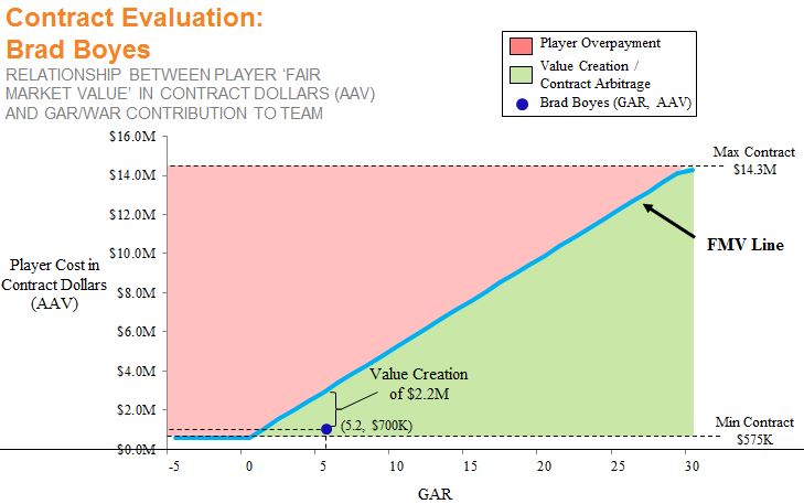
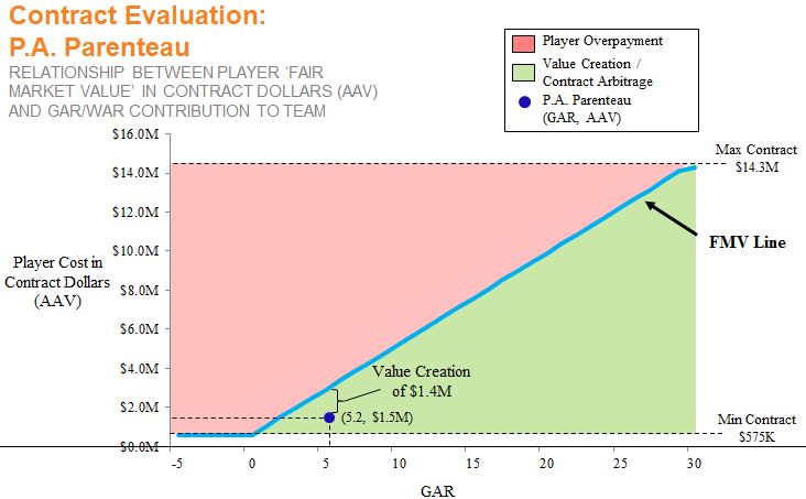
As the charts above show, given the fact that a ~5 GAR player is typically worth $2.9M, as long as Parenteau and Boyes perform in line with their recent history, the Leafs will have immediately created a combined $3.6M in salary cap value when they signed these two players. Further, being more than halfway into the season, the value that Pierre-Alexandre has brought on the ice thus far speaks for itself. Finally, none of this analysis even factors in the potential ‘exit’ value that Lamoriello & Co. could pick up by offloading P.A. or Brad for picks or prospects at the deadline, which is hopefully made easier by their very minor cap requirements.

Conclusion

To wrap up, the great work done by the likes of Hawerchuk and Eric Tulsky has provided us with the perfect framework to dig deeper into using GAR to quantify player value. Hopefully this article has been helpful to walk through those concepts, illustrate what this relationship looks like visually, and to show how the Cap Efficiency Curve can be a useful tool for analysis of player contracts and salary negotiations.

Building on these concepts, within the constraints of the CBA, the most legitimate, ‘fair’, and repeatable way for a team to maximize their cap efficiency is to either focus on acquiring young players in the draft, or by trying to trade for prospects early into their tenures as NHLers. As such, the upcoming third part of this series will focus on how teams can take advantage of Entry Level Contracts and Restricted Free Agency to consistently generate contract arbitrage opportunities for themselves, and maximize their wins per cap dollar spent.

Understanding ‘WAR’ and its Practical Applications to Player Evaluation (Part 1)

(OSA’s WAR ‘Explainer’ – Part 1)

This article is being co-posted on Maple Leafs Hot Stove as well as on my own site, http://www.originalsixanalytics.com. Find me @michael_zsolt on twitter.

@DTMAboutHeart of Hockey-Graphs.com and I recently exchanged tweets about the ‘WAR’ metric.

Twitter Exchange

Twitter Exchange pt2

This exchange brought to my attention that, despite the great work that has been done by the creators of WAR, it is a very complex metric. As a result, many don’t know exactly what ‘Wins Above Replacement’ (WAR) is, or how it works in hockey. It also struck me that, currently, much of the hockey community falls into one of two groups:

  1. Those who don’t know about, or fully understand WAR (or similar metrics), and thus ignore them, and
  2. Those who understand WAR, but think it is not yet developed enough to fulfill the original single number dream

(As well as perhaps a third group: teams that are secretly using WAR but not telling anyone… possibly evidenced by the creators of WAR now both being employed by professional sports teams).

As such, I am writing this series as an attempt to amplify the work done in this area. My main objectives are to increase the number of people in the conversation, as well as to demonstrate some of the practical applications, and limitations, of using the WAR metric to evaluate players. I will be focusing solely on the WAR metric developed in 2014/2015 by the great team at WAR-On-Ice.com (WOI), who are sadly leaving the public hockey world on March 31st, 2016. For those who don’t know, they are providing access to their entire database’s raw data up until that date. For reference beyond March, I have also uploaded their raw WAR/GAR by season output to my own website.

Further credit is owed to Tom Awad’s work on ‘Goals Versus Threshold’, a very similar stat that the WOI ‘WAR’ metric built upon. Last, I also want to give credit to Moneypuck’s excellent 2015 ‘Building a Contender’ series, where he applied GAR to building a winning franchise, which I have cited multiple times in article below.

So – before I get into WAR itself – why should you care?

Why is WAR Important?

I don’t think anyone will disagree with the following:

  1. The purpose of hockey is to win the game
  2. A team wins the game by scoring more goals than its opponent
  3. A player’s ‘ultimate’ contribution to his team is defined by his ability to improve his team’s goal differential (e.g. to increase goals scored and decrease goals against)

Although these three things are very basic, they are the foundation of why WAR is an important metric. It is easy to evaluate players strictly on the stats everyone has readily available: Goals, Points, Assists, etc. However, the classic example of where these fall short is the high-flying scorer who gives up two shots/goals against for every one that he gets. Corsi has become very popular for addressing this through an adjusted, game state-specific plus/minus, based on shot attempts. Although Corsi and WAR are built off similar concepts, ‘WAR’ tries to take shot rate metrics like Corsi, combine them with other factors, and then tie the result directly to the column on the score-sheet that matters the most: Wins.

What is WAR?

As mentioned, ‘WAR’ is a metric that attempts to combine a player’s contributions in offensive, defensive, and other aspects of the game, into the number of ‘Wins’ he contributes to his team. A fundamental concept of WAR is that it constantly compares NHL players to a set of ‘baseline’ expectations. This baseline is similar to looking performance versus league average, though it ends up closer to the league ‘minimum’.

Baseline expectations are important because of player value, and cost: an NHL team should only pay more than a bottom-tier salary if a player is contributing more than bottom-tier results. Thus, ‘baseline’ (or ‘replacement’) level players represent the quality of player that could be acquired for relatively little salary/cost on the free agent or trade markets. WOI calls their method the ‘Poor Man’s Replacement’, as they derive it based on players who have limited NHL experience. Conceptually, these are the players called-up to fill a 3rd/4th line role when injuries require it.

Finally, in order for WAR to convert performance into wins, we must first derive ‘goals’ contributed. Eric T has shown that roughly ~6 goals = 1 win – directly connecting goals above baseline into wins. Ironically, many people have now realized that ‘Goals Above Replacement’, or ‘GAR’, is actually easier to interpret than WAR, especially for individual players. As a result, from here on I will largely focus on GAR, though you should keep in mind that the two metrics are interchangeable at the rate of 6:1.

One last comment before the data…

A Caveat on ‘Catch-All’ Stats in Hockey:

As Michael Lewis’ Moneyball has shown the world, Baseball is the perfect sport for a WAR-type metric. Hitting, fielding and pitching all arguably equate to individual skills disguised within a team game, easily allowing statisticians to separate out individual contributions versus context, and noise.

Hockey, on the other hand, is a sport where it is very difficult to create a single statistic that will summarize ‘all’ of a player’s contribution in one number. As illustrated in this helpful post by Eric T from 2013, it can (conceptually) be almost impossible to perfectly adjust for all aspects of the game at once. However, those who have trudged through the Road to WAR series will see the extreme amount of adjusting for context that WOI has done, where they simultaneously controlled for teammates, opponents, game-state, and many other things – getting all the way down to elements as seemingly minor as travel fatigue (e.g. home/away team performance, and impact of playing on back to back nights). This level of detail and rigor suggests to me that WAR is among the most advanced publicly available stats to date.

Regardless of if you choose to place much value on WAR/GAR, I want to emphasize that no metric will ever justify ignoring other methods of player evaluation. Given WAR/GAR says nothing of a player’s role, Rob Vollman’s player usage charts are a very complementary tool to use alongside it. I also encourage the uninitiated to check out Eric T’s straightforward primer on different metrics that can be used for player evaluation.

Now – back to GAR, and finally, some actual numbers.

What is a ‘good’ GAR/WAR score versus a bad one?

At a high level:

  • If a player has a ‘GAR’ of zero – they are equivalent to a baseline/replacement level player
  • If a player has a positive GAR, they are ‘better’ (at contributing to their team’s goal differential) than a baseline player
  • If a player has a negative GAR, they are worse than a baseline player

In order to be a bit more specific, let’s look at some data from Moneypuck’s series, which was very insightful on this front. His third article looks at:

  1. The GAR scores of every NHL player from each season in his sample
  2. The GAR scores of the players from the four conference finalist teams each year

The two charts below summarize his data.

( Note: I haven’t made any changes to his data – these are the same numbers shown in a different format)

GAR Distribution - All Players

Top Team - Player Count by GAR

From this data we can make a few observations:

  • It is very difficult for a player to pass a GAR score of even 10 in a given season
    • The first chart shows that fewer than 14% of players achieve this each year, and the second shows that even conference final-reaching teams usually only have ~4.5 players with a GAR of 10+
  • Even fewer have a GAR of 15+, at approximately 5.9%, or only 1 in 17 players in the league
  • Last – as highlighted on the first graph – over 70% of the seasons played in the NHL score a GAR of 5 or lower
    • Put differently, 70% of NHL players fluctuate in and around the league minimum level of contribution to their team’s goal-differential

Now, in order to illustrate how various players are scoring in terms of GAR – I have summarized the following table for you to compare against your own, personal eye-test.

Example Players by GAR Range

Hopefully this table helps to set some benchmarks in your own mind about how various players score on GAR. This table also makes it clear that Goalies and Defensemen are under-represented in the top GAR ranges, when looked at on a three-year average basis. This highlights an important qualifier of the GAR metric: like most NHL player evaluation, it currently best evaluates a player’s offensive contributions.

Looking at the components of GAR (the next section) will explain why: defensemen will largely contribute to just one or two of the six components (e.g. impact on shot rates), while forwards will contribute to shot rates while also providing material contribution through their shooting percentage, face-offs, and penalty drawing. As a result, when using the current GAR metric to evaluate players, it will be most accurate to compare players within positions, rather than across them. For what it’s worth, WOI previously hoped to add other defensive components to WAR, as well as a measure of play-making ability, helping to offset this gap. However, the closure of their site means these areas will not be publicly incorporated until another brave statistician picks up where they left off.

Now that we know why GAR is important, what a good/bad score is, and who typically scores where – what factors is this number actually considering?

What Are the Components of GAR/WAR?

 As WAR-On-Ice has already given a very detailed summary of the math behind the metric, I’ll instead focus on the big picture of its component parts. WAR is currently made up of the following six components for skaters, which I have grouped into the three broad categories below:

Offensive Contributions

  • Shot rate for
  • Shooting percentage

Defensive Contributions

  • Shot rate against

‘Gameplay’ Contributions

  • Faceoff win percentage
  • Ability to draw penalties
  • Ability to avoid taking penalties

Whether or not you are familiar with statistics, I think most of us can agree that increasing your team’s shot rate differential, shooting percentage, faceoff percentage, and power play opportunities, while decreasing your team’s minutes on the penalty kill, are all going to help contribute to goals and wins. As a reminder, each of these have their own definition of ‘replacement level’ that GAR is calculated against. One last side note: Goalies are calculated as their own category, based on Sv%, which I have omitted here.

Now, the fun part: 

How to Analyze a Player’s WAR/GAR – A Case Study

In order to demonstrate the various components of GAR, I have chosen a player that we all know, and who also happens to contribute at both ends of the ice: star two-way center, Jonathan Toews.

Looking at Toews’ GAR metrics in the 2013-2014 season gives us the following:

Toews 6 bars

Keep in mind: across all components, a positive GAR is a better result. E.g., Toews’ positive ‘Shot Rate Against’ GAR score (3.6) means he has been successful in reducing shot attempts against.

The above data shows us that:

  • Although Toews is a major offensive threat, a significant amount of his impact comes from his defensive and ‘gameplay’ contributions, e.g. shot suppression, face-offs, and ability not to take penalties
  • In 2013-14 Toews won more than half a game (e.g. ~3 GAR) in his face-off percentage alone, putting him among the leagues’ best
  • Toews contributes most offense through his possession and shot-attempt driving capabilities (shot-rate), rather than by being a sniper
    • In contrast, while not shown here, Patrick Kane contributes more through his strong shooting percentage, often scoring 6-7 GAR per season in Sh% alone

Introducing a style of chart I will label ‘GAR Bars’, we can summarize a player’s total GAR contribution back into those three major categories:

Toews 2013-2014 GAR BAR 

This chart shows the exact same data as the prior one; the only difference is that now I have aggregated each of the six components into their general buckets. For two final illustrations, we can expand on this bar to analyze Toews based on his GAR over time. The charts below show (i) Toews’ absolute GAR contribution over a number of seasons, as well as (ii) Toews’ relative GAR contribution, showing each category as a portion of his total.

Historical Absolute GAR

Toews Historical Absolute GAR

This chart shows us that:

  • Toews has been in the 20-25 GAR range for most of his career – an extremely high score, especially when considering only 2.4% of all NHL seasons exceed 20 GAR
  • Despite winning the cup in 2014-2015, Toews’ individual performance last season dropped to his lowest level since his rookie year
    • While ~16 is still a very good score, this decline may be indicating signs of Toews’ age, suggesting we should expect a slightly reduced level of performance from him going forwards

Historical GAR Distribution

Toews Historical Relative GAR

Finally, looking at Toews’ GAR contribution by category shows us the biggest step down in 2014-2015 was in his defensive play. Although I haven’t watched enough Blackhawks games to observe this myself, one reason this could be happening is a slight decline in skating ability/speed with age, preventing him from being as involved around the rink as he once was.

Conclusion

Now, I haven’t used this data to hammer home a unique point of view about Toews – no one needed me to quantify it to know he is a future Hall of Fame-caliber player. Rather, the point of this article has been to provide some colour behind the basics of the WAR/GAR metric, and to illustrate in a simple, straightforward manner how anyone could apply this metric to their own thinking on player evaluation.

Regardless, it is clear that Jonathan Toews is a hugely valuable player to Chicago at both ends of the ice, sitting in the elite, 20+ GAR echelon, and having peers among the likes of Crosby, Kopitar, and Ovechkin. This analysis also says nothing about the leadership skills he has demonstrated on and off the ice, taking his team to an unprecedented three cup wins in the last six years. As a result, I think we all believe that Captain Serious earns every dollar of his $10.5M cap hit. But how can we know for sure? Unfortunately – for that, you’ll have to wait for the next installment of the series, where I will demonstrate how to use WAR/GAR to quantify what a player is worth.


What Draft Round Can Tell Us About a Player’s Expected Long Term Performance and Development (Part 1)

This article is being posted here as well as in parallel as a guest post at Maple Leaf Hotstove. FYI, for those who read my last post – as promised – this article is a succinct summary of my draft analysis ‘report’ shared earlier. 

The hockey analytics community has looked at many aspects when projecting a player’s performance over their career: prior league, prior scoring rate, performance of players with similar characteristics, size, and date of birth – amongst others. One example of such work was an article from earlier this year by ‘moneypuck’ at NHLnumbers.com.

Moneypuck’s analysis derives its foundation from an excellent study by Michael Shuckers in 2011, where Shuckers was one of the first to create a standardized view of ‘draft pick value’. The quality of Schuckers’ analysis drove many other authors to do work that followed suit, building on his approach. However, in his paper, Michael chose to define ‘draft pick value’ entirely based on likelihood to play >200 games in the league. Although that is a reasonable metric – and few would argue that reaching 200 NHL games means a draft pick was NOT successful – there are limits to using only a single metric to define ‘success’.

How ‘successful’ a pick was, and the ensuing value of a draft pick, is highly sensitive to how we choose to define success. Is a pick successful after 40 games, 80, or 200? Are they successful after 30 career points, or 100? How about their points per game? Or their total career points? How would our definition of ‘success’ change on each of these metrics if they are a forward or a defenseman?

As you can imagine – this isn’t a simple thing to answer. Earlier in 2015, Stephen Burtch did some interesting work down this path, where he combined expected GP with expected Pts/Gm to create a new draft pick value figure – which was a big step in the right direction. However, even Pts/Gm has its gaps, given that it only considers players still in the league. As time goes on, the least successful players will leave the league sooner, increasing the average Pts/Gm of those remaining. In a perfect world, we would want a metric that has already been adjusted for a player’s likelihood to succeed in the league, rather than one based on his success if he can stay in the league. (Though – to be fair – Burtch does seek to address this point through multiplying probability of reaching 200 games by expected Pts/Gm).

In order to address these points, I have taken a very detailed look at long term player performance and development based on draft round, incorporating a wide range of metrics into my analysis. Specifically, I have reviewed the five years of players drafted from 2000-2004, as well as the ensuing 9-13 years of NHL season data.

Arguably the biggest factor in whether or not analysis is put into practice is if a team’s front office and coaching staff truly understand it, and believe the results of the analysis enough to buy-in to it – which will often come down to the method by which that analysis is communicated. As such, I have tried to simplify the statistical methodology involved in this work, and display the output visually in a way that is easily understood and hopefully very accessible to stats and non-stats folks alike.

(As a note – this article focuses strictly on metrics related to player performance and development. However, a natural follow on to this is then connecting that information to draft pick value, as mentioned, and after that, how successful teams have been in drafting – both of which are covered in my full report, originally posted here). 

What I Hope To Answer

The objective of this analysis is to investigate ‘typical’ player performance and development trajectory after being drafted in a given round, in order to answer the following three questions:

  • If a player is drafted in round X, and is ultimately able to make the NHL, by when should they be expected to be a contributing NHL player?
  • How well does the typical player perform over the course of his career (on various metrics) after being selected in a given round?
  • Within the first round, how do the top 10 overall picks perform versus those taken 11th-30th?

So – let’s get into it.

Analysis of Long Term Player Performance and Development by Draft Round

I have split out the upcoming sections of analysis by each type of metric used. I will then revisit the three questions above directly in the final section on conclusions.

Games Played Thresholds

As Michael Shuckers showed very clearly – players drafted in the first 2-3 rounds are much more likely to appear in the NHL; however, the likelihood of a playing one or more full seasons diminishes substantially after the first round

Games Played Pic 1

Games Played Pic 2

In terms of player development, this data suggests that:

  • If a 1st round pick hasn’t played a game by their fourth potential NHL season, they likely will never appear in the NHL
  • 20-30% of successful 2nd and 3rd round players only begin to meaningfully play for their franchise between 5-7 years after being drafted (e.g. the pink shaded area on the ’80 games played’ chart)
  • The gap between the top 10 overall and the rest of the first round is actually relatively small when looking at the likelihood to pass the 150 game threshold (especially in comparison to metrics later in the article)
  • And, as we know – all other rounds after the first three appear to have close to equal likelihoods of producing long term NHL players

Points / GM Data

Forwards taken in the top 10 overall show an unbelievable ability to outperform in P/GM over their careers (which Stephen Burtch has shown is even more distributed within the top 10¸ where the top 1-3 picks overall are meaningfully better than picks 4-10)

Pts per Game - F

  • Interestingly, 2nd and 3rd round forwards tend to increase their per-game output over time, largely converging with players drafted 11th-30th overall
  • However, given this metric is an average of those still playing, there will be a survivorship bias that partially drives this effect
    • E.g. Low producers will leave the league more quickly, increasing the average for those remaining – as shown by the fact that 30% of the players shown are from Rd 1 in season ‘6’, this increases to 40% by season ‘10’
    • This data can more reasonably be said to tell us that, in order to stay in the NHL over the long term, a forward must achieve a minimum of roughly 0.20 points per game

Defensemen naturally display a much more narrow distribution of results, accounting for the fact that a ‘strong’ defenseman will not always play a significant point-scoring role

 Pts per Game - D

  • P/GM data for defensemen is not terribly insightful, but I have included it in order to provide the data for those interested
  • One note – If you look closely, you can see surprisingly strong (and erratic) performance of Round 5 defensemen – starting very weak (no points registered in season ‘2’), but then ultimately being among the highest points per game in seasons ‘5’ through ‘10’
    • This particular point is driven by a small sample size issue: 49 D were drafted in the 5th round, but only a handful played many games – three of whom happen to be John-Michael Liles, Kevin Bieksa, and James Wisniewski

Points Scored Thresholds

A player’s likelihood to surpass the 30-point threshold tends to resemble their likelihood to pass ~150 career games played…

Pts Threshold Pic 1

… However, players drafted in the third round fall behind in terms of likelihood to pass the 100-point career threshold

Pts Threshold Pic 2

  • Where earlier charts show strong similarities between the long term potential of 2nd and 3rd round players, the ability of those taken in the 2nd round to break the 100-point career threshold is a clear differentiator between the two
  • Based on this, teams may do well to target top scorers in rounds 1 and 2, before moving to defensemen, shut down forwards and goalies in the third round and onwards
  • Again, top 10 overall picks differentiate themselves here as well, with over 70% passing 100 career points

Cumulative Career Points

The ideal metric to compare performance by round must be adjusted for players with limited NHL careers – which brings me to Lifetime Production, or Cumulative Career Points Scored

Lifetime Production - F

Lifetime Production - D

(Note – Forwards and Defensemen are shown on different scales)


  • Here, 1st round picks wildly outperform all others, showing that the combined skill and typical longevity of even a mid-to-late 1st round player (11th-30th) will equate to an average 159 points over 10 seasons for forwards, and 105 points over the same timeframe for defensemen
  • This compares to the significantly lower 68 average career points for second round forwards, and 44 average career points for second round defense
  • Notably, third round forwards also re-assert their value here, showing that – although they will only typically produce a total of 36 points over 10 seasons – they still will consistently outperform rounds 4-9 in career points

Drawing Some Conclusions

Having now walked through each chart and its meaning, I want to summarize my findings from above. To do so, let’s revisit the original list of three questions:

If a player is drafted in round X, and is ultimately able to make the NHL, by when should they be expected to be a contributing NHL player?

  • First round players typically make their initial NHL appearance within 1-2 years, and will almost always have played their first full season (~80 games) by their fourth year after being drafted
  • 2nd and 3rd round players take much longer to develop, and many only play a full season by their 5th-7th years after being drafted
  • Players who haven’t played by these general timelines become highly unlikely to ever make serious NHL contributions (>1 season played)

How well does the typical player perform over the course of his career (on various metrics) after being selected in a given round?

  • Most players drafted outside the first round never make the league at all (2nd round players have a 60% likelihood of playing one game, and a 35% likelihood of playing a full season; for 3rd round players, closer to 40% play one game, and only 28% play a full season)
  • Based on their combined likelihood to play 2+ NHL seasons, score 30+ NHL points, and reach 0.4-0.5 or more pts/gm, 1st, 2nd and 3rd round players are the only players with a meaningfully higher likelihood in succeeding in the league
  • However, based on the likelihood to score >100 NHL points, 1st and 2nd round players are able to separate themselves from the 3rd round as well

Within the first round, how do the top 10 overall picks perform versus those taken 11th-30th?

  • The top 10 overall picks are significantly more capable than all others, even versus their first round peers
  • Over 70% of top 10 overall picks pass 100 career points, typically after ~6 seasons, versus 50% of those picked 11th-30th, who often take 9-10 years or more
  • Only forwards taken in the top 10 overall can truly be expected to score 0.6-0.7 pts/gm or more over their careers (although there are many examples of players who perform at this level of production that were taken outside the top 10, such as Ryan Getzlaf and Corey Perry)
  • In a hypothetical trade for active players, a ‘typical’ top-10 overall pick should be treated as likely reaching >350 career points as a F, or >170 as a D – thus, one-for-one, a team should be expecting to get a true star player in return if they are giving up a potential top 10 overall pick

In the end…

The long term performance expected of a player based on their draft round is something that is highly relevant to teams throughout their decisions in trades, on draft day, and in supporting a player’s development over his career. Hopefully you have found this analysis to be interesting, and found that the work was also able to build upon what is already out there by expanding the range of metrics that we look at. As mentioned, the PDF I linked to above also begins to apply this to both a revised (and straightforward) metric of draft pick value, as well as to answer the question of ‘Which teams were the most successful?’ in the draft years studied. Keep an eye out for ‘Part 2’ of this article – where I apply the data above to the trades done by the Leafs on Draft Day last summer, in order to see if Hunter, Dubas and friends were winners or losers in their exciting deals…

This article is presented by OAK Coasters, a website where you can by beautifully crafted, hand made One of A Kind (OAK) coasters that make the perfect gift. Check them out at OAKCoasters.com.